In my last post, I gave a quick and dirty explanation of the principles of precise GPS positioning. In it, I mentioned the double differenced dual-frequency phases as the main observations behind RTK positioning. However, that wasn’t very informative for those out there who have little knowledge of such terminology. So hopefully, the next few blogs will elucidate my ramblings for those out there who may actually be interested :).
A couple of FYI’s before I begin.
1. I’ll be using the same notation as Wellenhof et al., and I recommend it for anyone interested in the principles of GPS…IMHO it’s the best book out there on the subject.
2. If you would like to test your own code, you’re more than welcome to use the test datasets which I’ve used.For the purposes of this study, I use observations from two Continuously Operating Reference Stations (CORS) in Ohio, which are located Southeast of Cleveland.The first site is OHLO, the second is ZOB1, and they are located ~1 km apart from each other, which is a typical baseline length for cm level positioning.
http://www.ngs.noaa.gov/cgi-cors/corsage.prl?site=OHLO
http://www.ngs.noaa.gov/cgi-cors/corsage.prl?site=ZOB1
If you click on “Standard Files”, you will be directed to the following NGS site (http://www.ngs.noaa.gov/CORS/standard1.shtml).The RINEX files can be downloaded for each observation site for a given date.
* Note, you will need the navigation files as well, which describe the position of the GPS satellites at different measurement epochs.
**If you can’t figure it out, send me a message and I’ll be glad to email the necessary files.
Okay, lets begin.
One of the most important factors in precise positioning applications is baseline length, i.e. the geometric distance between the two GPS receivers. With short baselines, certain simplifications/assumptions can be made due in notation, due to similarities in the ionospheric and tropospheric path that both signals had to pass through as they traveled towards earth. As the baseline length increases, these simplifications are no longer valid, but for our purposes (short baseline), they are sufficient.
The double difference observation for short baselines is given in the following notation.

Where


Note that for dual frequency receivers, we could form this operation on both frequencies, i.e. L1 and L2.Often, authors will refer to 
Assuming we correctly read in the observations from the RINEX file, what do we do next? Well, we must first compute an approximate location for the roving receiver, because this location is embedded in the geometry term of the above equation. For starters, we could use the known position of the base station. Remember that we assume one of the receivers to be located at a known position (base station), because we will need to hold that position fixed in order to estimate the location of the other receiver(rover). With an approximate location of the rover estimated, and a sufficient amount of observations, we can solve for our unknowns via a least squares solution (LSS). Because the equation above is non-linear, we linearize it about the approximate receiver location, and solve for the unknowns, which are


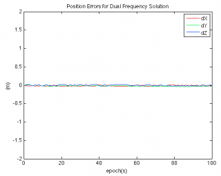
Assuming we have done everything correctly, we will have what is known as a float solution. Because least squares doesn’t know any better, it estimates the integer ambiguities to be real-valued numbers, which we know to be untrue. The accuracy of the float solution is shown below for 100 epochs of data.

Looking at the figure above, we can see the accuracy of the float solution is generally on the order of 0.5-2m, a significant improvement from absolute positioning. However, its not 2-5 cm accuracy we expect from survey grade GPS receivers! So how do we improve the float solution so that we can achieve higher accuracies(such as the plot below)?
Stay tuned!

Very well explained. Any difficulties/problems you had in computing the float solution?
Lots of difficulties, mainly due to coding blunders, or wrong signage :). In theory however, the LSS is pretty straightforward.
I have the double-differenced phase measurement from two satellites (j,k) and two receivers (A,B). But can you please explain with example how to compute float solution using Least square principle….I am struck up there
The float solution is calculated by adding additional unknowns to the linearized system of equations.
You mentioned two satellites and two receivers. Is that all the data that you have? In the case of GPS, there is commonly between 7-10 satellites in view at any given point in time. Is the position of one of the receivers known?
In any case, for each satellite, the position is known (or at least we can assume that it is known for now). Also, lets assume the position of receiver 1 (a base station) is also known. That means for our double-differenced (2 satellite/2 receiver combination), there is a total of one observation, but 4 unknowns. The observation is the double differenced phase between the two satellites/receivers, the unknowns are 1.) the 3D baseline vector between receiver 1 and 2 (3 unknowns), and 2.) the unknown double differenced integer ambiguity. Therefore, it’s impossible to compute a float solution using just two satellites/receivers. Furthermore, it’s impossible to compute a float solution from a single epoch, you need multiple epochs which you can leverage by knowing the the unknown integer ambiguities don’t change from epoch to epoch (well, very rarely…cycle slips are possible).
To summarize, you need a minimum of four satellites and two epochs to compute a float solution. In my examples shown on the blog, i believe that i used 100 epochs at 8 satellites to compute the float solution.
Somehow I missed reading your reply in time.
I thank you very much for your kind reply and all very useful posts.
I am still struggling in developing covariance matrix. Can you please explain how to develop a covariance matrix of double differences.
I have data from almost 8 to 13 satellite data from Rinex observation file of two stations. But I have taken top two satellites w.r.to availability of highest no of epochs. Both the receiver positions are known from Rinex observation files. According to papers from Tuenissen, Blewitt like authors, the double difference is calculated between two satellites and two receivers…..
but a double difference between two satellites and two receivers give only a single column DD( double diff) data…for which a co-variance matrix can’t be calculated….can you suggest me please…how to get covariance matrix
Could you explain what GPS float is?
Yuan,
“GPS Float” refers to a common least squares solution for GPS/GLONASS positioning. In order to do high accuracy positioning (cm level), we must resolve the correct integer amount of carrier phase (L1 and/or L2) cycles between the reference satellite and our GPS receiver. This unknown integer amount of cycles is referred to as the integer ambiguity in typical textbooks. There is only one true integer, and we must know what it is for each satellite in order to get cm level accuracy.
The GPS float solution is often used as the first step towards finding the true integer. Once you’ve computed the GPS float solution, you can use the estimated integer ambiguities and their associated covariance matrices in a program like LAMBDA to find the true integers.
To recap, using the psuedorange and carrier phase measurements (which ive described in my post), we estimate the unknown integers and position in a least squares solution. However, the least squares solution doesn’t estimate the integer ambiguity as an integer, rather as a real number. For example, if the correct integer amount of carrier phase cycles was 24, the GPS float solution might estimate the integer as 23.873, a real valued number. The position accuracy of the GPS float solution is ~.5 meters, which may be good enough for your particular task. However, if you would like cm level accuracy, you will have to correctly resolve the integer ambiguities.
Excellent post, need more on this. I find that many articles and papers about ambiguity resolution never touch on the float solution. However, for people without background in least squares and the concept of an overdetermined system, the process of obtaining a float solution may not be so intuitive.
What would really be great IMO, if you could add to your post, the least squares process. As in stepwise, how you derived your design matrix, how many epochs you used, what observations you used (code/carrier phase), etc. I am a fellow geomatics engineering graduate student, and I am happy to see such blog posts and would like to help in anyway possible.
Thank you very much for providing this information. I am reading the other posts you have here. It is excellent work.
Thanks Eric. It’s been a while since I’ve worked on this, but perhaps it would be valuable to post the code. It was all written in matlab so it should be relatively easy to follow. If someone wanted to take it and run with it (or better yet, translate it to python), it could be a really nice contribution to existing open source toolboxes, like Easy Suite.
It will be a great help to all of us if you can contribute the stepwise process of ambiguity estimation . Easy suite and LAMBDA Matlab code do not give details how to develop design matrix and covariance matrix…your stepwise guidance will be a great help to students like us. Thanking you in advance!
I agree, I can see that you worked on this about 5 years ago. Perhaps, posting the code might be helpful as well. After all, the code would show the way you formed the design matrix and other details.
We are grateful to you Eric for your help and knowledge sharing nature!
Million thanks! Your code may surely make us understand better the process of ambiguity estimation and removal. I acknowledge your great help.
(mistaken Eric as Clpxosu…excuse me pl.)
We are grateful to you Clpxosu, for your help and knowledge sharing nature!
Million thanks! Your code may surely make us understand better the process of ambiguity estimation and removal. I acknowledge your great help.