Okay, since those of you who are reading this are probably wondering if I’m interested in anything else besides high accuracy GPS processing…the answer is yes! I’ve just been sort of consumed with the GPS project, which is nearing completion (at least in my head). I’ll probably throw up one more post explaining how to step into the narrowlane linear phase combination from the widelane, or maybe how to detect cycle slips, but other than that, it is basically complete!

Because I’m also interested in photogrammetry, the next “project” will be related to installing/learning/applying openCV, which is an open source image processing library. You can read more about it here (http://opencv.org/). Since I am somewhat of novice Linux/Unix user, it took a while to figure out how to install correctly on my machine. Hopefully this tutorial will help you mitigate some of the mistakes that I made as i went along. I meant to include photos to go along with this, but forgot…so hopefully the text will be enough.

1. Download source – johndoe$ git clone https://github.com/Itseez/opencv.git (you will also need cmake)
2. Install cmake within opencv folder – opencv johndoe$ sudo port install cmake
3. Make a new folder/director called build within the opencv directory – opencv johndoe$ mkdir build
4. Type the following command – build johndoe$ cmake -G “Unix Makefiles” .. (after running, you should get “build files have been written to”
5. Type the following command – build johndoe$ make -j8 (this makes the your unit work!)
7. Type the following command – build johndoe$ sudo make install (install openCV)

It might take a while to get through steps 1-7, so don’t give up too quickly!

Since this blog isn’t totally devoted to technical topics, I thought i would post several photos from my trip to Colorado during spring break. Thanks for the hospitality Boris, Dave, and Rachana!

Without further ado…

Skiing at Keystone
IMG_0600

Coors Brewery Tour
IMG_0601

Pikes Peak
IMG_0612

Royal Arch
IMG_0615

Okay, I had some problems in the last post correctly resolving the true fixed ambiguities from the dual frequency GPS phase measurements. Well, I think I’ve resolved them finally! I took a different approach to the least squares solution, and after running the estimated ambiguities and a posteriori covariance matrix through LAMBDA, I was able to obtain the correct integer ambiguities (for the most part). As can be seen below, there are a few instances in which the INCORRECT integers are estimated, which corresponds to a significant increase in the errors associated with the LSS solution.

Screen Shot 2013-03-16 at 4.04.09 PM

Screen Shot 2013-03-16 at 4.02.35 PM

As can be seen, the absolute error of the fixed ambiguity widelane solution is on the order of 10-15 cm. However, when the integers are incorrectly estimated, the errors are much larger, approaching ~ 5-7 meters in magnitude. I haven’t examined exactly why I am incorrectly estimating the widelane ambiguities between the 25th and 30th epoch, but that may be a topic for later… I can tell you, however, what things i changed which allowed me to get correctly estimate the integer ambiguities most of the time.

Essentially, instead of providing a priori estimates of N for the LSS solution, I carried each of the ambiguities as unknown parameters in the adjustment. The a posteriori covariance matrix was derived from the LSS as described in earlier posts. The float solution associated with the widelane linear combination is fairly noisy, as can be seen below, and though the float integer estimates are generally consistent, some are actually biased by a wavelength or two.

Screen Shot 2013-03-16 at 10.53.46 AM

Screen Shot 2013-03-16 at 4.45.31 PM

Once the widelane ambiguities have been resolved, the L1 ambiguities can be derived in the following manner for short baselines

N_{L1} = \Phi_{L1} - f_{L1}/f_{WL} *((\Phi_{WL} - N_{WL})

For longer baselines, we must include the ionospheric contribution

N_{L1} = \Phi_{L1} - f_{L1}/f_{WL} *((\Phi_{WL} - N_{WL}) + b*((f_{L1} + f{L2})/(f_{L1}*f_{L2})

The L2 ambiguities can be derived in an analogous way by exchanging the roles of L1 and L2 in the equation above. Once the L1 and L2 ambiguities are resolved, the narrowline ambiguity is easily obtained, and this is the linear frequency combination that is most often used in commercial survey grade GPS receivers.

In previous bloggings on precision GPS, we have assumed the measurements (both code and carrier), to be uncorrelated. In particular, the covariance of the carrier phase measurements at an instant was modeled as
\Sigma_\phi=\sigma_\phi^2 I
and for pseudorange measurements, we had the following
\Sigma_\rho=\sigma_\rho^2 I
In our error model,
\sigma_\phi =0.025 cycles
\sigma_\rho = 3 meters
I = Identity \ matrix
So, for example, if we are talking about widelane measurements, the corresponding cycle error expressed in units of range would be
0.025 cycles*.86 m/cycle = 0.0215m
However, correlation between double differences exist, and we will examine and hopefully exploit those below for the purposes of resolving our ambiguities.

According to Misra and Enge (Eqn 7.65), the (K-1)x(K-1) covariance matrix for K satellites would have 2’s on the main diagonal and ones in all off-diagonal positions. I’m still trying to implement matrices into wordpress (with little success), so i will just use MATLAB notation. The covariance for a pair of double differences (DD) would have the following notation.
\Sigma_\phi ^{DD} =2 \sigma_\phi^2 \left[  \begin {array}{ccc}  2&1\\  \noalign{\medskip}  1&2  \end {array}  \right]

Which then becomes
\Sigma_\phi ^{DD} = \sigma_\phi^2 \left[  \begin {array}{ccc}  4&2\\  \noalign{\medskip}  2&4  \end {array}  \right]
Okay, now lets begin the LAMBDA process.

1. Obtain float solutions and disregard the integer constraint on the ambiguities. Note the we use the covariance matrix which we described above in the LSS solution process (actually its inverse)

l=Ax
x= (A^T * (\Sigma_\phi ^{DD})^{-1} * A)^{-1} * (A^{T} * (\Sigma_\phi ^{DD})^{-1} * l)

By the law of covariance propagation, the corresponding covariance matrix for the estimated parameters would be
\Sigma_{xhat} = (A^T * (\Sigma_\phi ^{DD})^{-1} * A)^{-1}

To compute the fixed ambiguities, LAMBDA needs two inputs, i.e. the estimated float ambiguities, and the estimated covariance matrix of the float ambiguities. I won’t get into the intricacies of LAMBDA technique at the moment, but I will show you the results. Unfortunately they are not correct!

The plot below shows the difference between the true integer ambiguities versus those estimated by LAMBDA, my initial float solution, and the revised float solution.

Screen Shot 2013-03-03 at 2.32.27 AM

As you can see, I only correctly resolve 2 out of the 7 ambiguities with LAMBDA…not very good! I have two hypothesis for this error.
1. Right now, i am assigning equal variance to each individual satellite for my stochastic model. However, perhaps i should change this as a function of elevation angle and/or signal to noise ratio?
2. Currently, i am using initial approximations for the float ambiguity measurements, which is derived from a excerpt in the Misra and Enge book. Maybe i will try the typical LSS method of assuming prior information on the float ambiguities and estimating them directly.

Either way, something needs to be done…

In my last post, i mainly described the steps involved in generating the well known GPS float solution. A surveyor is likely familiar with the float solution, as this is the type of positioning that is done immediately upon turning on the rover, or perhaps when one ventures to close to an overhead obstruction (such as a tree). In my field experience, upon starting up the rover, it usually took anywhere from 15 seconds to a couple minutes of a float solution before RTK could be achieved. They tell me that with the new receivers nowadays, the integer fixing only takes a few seconds, but I’ll have to see it first, before I believe it :).

Lets start where we left off last time, i.e. the float solution. As we’ve shown below the accuracy of the float solution is ~0.5-2 meters.
float

Additionally, recall that when we compute our least squares solution (LSS) with the double differenced phase measurements, we estimate the double differenced integer combinations, in addition to our unknown DX, DY, and DZ. I’ve included a plot below of the estimated DD integer combinations via LSS.

N_est

Notice how the estimated ambiguities jump around, yet seem to be be fairly stable (not drifting)? This is because the estimated integer ambiguities are estimated as real valued numbers from LSS! We know this to not be true however, THEY MUST BE INTEGERS! So, how do we go about fixing the float ambiguities to their true fixed values? And more importantly, how do we do precise GPS positioning once they are fixed? To do this, we’ll have to learn about linear phase combinations, which can be obtained from dual frequency GPS data. NOTE, if you have a single frequency (L1) receiver, the following section will NOT pertain to you. There is existing literature that pertains to ambiguity fixing via single frequency receivers, but it will not be covered below (at least not now, that is).

Linear Combinations

We are working with dual frequency GPS observations (L1 and L2). Linear combinations of two phases \varphi _1 and \varphi _1 can be combined to form an observation in the following manner
\varphi _{obs} = n_1 \varphi _1 + n_2 \varphi _2
Where n_1 and n_2 are arbitrary numbers, such as 1 and -1, 1 and 2, etc. Whenever we form a linear phase combination, it is imperative that we compute the correct wavelength of the linear combination! Remember the basic physics equation that relates wavelength to frequency
\lambda = c/f where \lambda is wavelength, c is the speed of light, and f is frequency. For a linear combination, the wavelength will be calculated using the following relationship.
\lambda = c/(n_1 f_1 + n_2 f_2)

The first, and arguably most important linear combination to be aware of is the so-called widelane combination. The widelane combination is very helpful in obtaining high accuracy GPS positioning due to its much desired longer wavelength. The longer the wavelength of the phase measurement, the greater the chance that you’ll be able correctly resolve the unknown integer ambiguity. Thus, as you may have guessed, the wavelength of widelane measurements is longer than that of the L1 or L2 measurements.

\varphi _{wl} = 1 \varphi_{L1} -1 \varphi_{L2} and \lambda_{wl} = 86.2 cm

Now, I must confess, I’m going to cheat on the next couple of posts…or at least this one. Remember the geometry term I talked about in the last post? In real life, the geometry term isn’t precisely known when the receiver is initialized, and that is why we use initial approximations for our least squares solution. However, for the purposes of clarity, I am going to use the true geometry value, and then back out the integer ambiguities from that. Once this has been done, we can go back to the “real life” situation where the geometry term is unknown, but for now, we will disregard that.

Using equation 9.31 from Wellenhof et al., we can estimate the widelane ambiguities. In the plot below, i show the estimated widelane ambiguities using the measured pseudoranges, as well as the true widelane ambiguities calculated with the true (without error) calculated pseudoranges.

Widelane_N

As can be seen, the widelane ambiguity estimates are much less noisy then the L1 estimates from the plot above. That being said, there is still noise (and bias) within the ambiguity estimate, so resolving them is not necessarily trivial.

TO BE CONTINUED

In my last post, I gave a quick and dirty explanation of the principles of precise GPS positioning. In it, I mentioned the double differenced dual-frequency phases as the main observations behind RTK positioning. However, that wasn’t very informative for those out there who have little knowledge of such terminology. So hopefully, the next few blogs will elucidate my ramblings for those out there who may actually be interested :).

A couple of FYI’s before I begin.

1. I’ll be using the same notation as Wellenhof et al., and I recommend it for anyone interested in the principles of GPS…IMHO it’s the best book out there on the subject.

2. If you would like to test your own code, you’re more than welcome to use the test datasets which I’ve used.For the purposes of this study, I use observations from two Continuously Operating Reference Stations (CORS) in Ohio, which are located Southeast of Cleveland.The first site is OHLO, the second is ZOB1, and they are located ~1 km apart from each other, which is a typical baseline length for cm level positioning.
http://www.ngs.noaa.gov/cgi-cors/corsage.prl?site=OHLO
http://www.ngs.noaa.gov/cgi-cors/corsage.prl?site=ZOB1
If you click on “Standard Files”, you will be directed to the following NGS site (http://www.ngs.noaa.gov/CORS/standard1.shtml.The) RINEX files can be downloaded for each observation site for a given date.
* Note, you will need the navigation files as well, which describe the position of the GPS satellites at different measurement epochs.
**If you can’t figure it out, send me a message and I’ll be glad to email the necessary files.

Okay, lets begin.

One of the most important factors in precise positioning applications is baseline length, i.e. the geometric distance between the two GPS receivers. With short baselines, certain simplifications/assumptions can be made due in notation, due to similarities in the ionospheric and tropospheric path that both signals had to pass through as they traveled towards earth. As the baseline length increases, these simplifications are no longer valid, but for our purposes (short baseline), they are sufficient.

The double difference observation for short baselines is given in the following notation.

\lambda\Phi ^{jk}_{AB}(t) = \rho ^{jk}_{AB}(t) + \lambda N ^{jk}_{AB} +noise

Where
\lambda is the wavelength of the frequency L1 or L2 frequency.
\Phi ^{jk}_{AB} is the double-differenced phase measurement from two satellites (j,k) and two receivers (A,B).
\rho ^{jk}_{AB} is the double-differenced geometric distance between the satellites in space and the receivers on the ground.
N is the double-differenced integer ambiguity of the phase measurements. It must be an integer! (e.g. 1, 3, 21, etc.)

Note that for dual frequency receivers, we could form this operation on both frequencies, i.e. L1 and L2.Often, authors will refer to \rho as the geometry term. As we will see in later posts, we need to know the geometry term to a certain degree of accuracy in order to resolve the integer ambiguities.

Assuming we correctly read in the observations from the RINEX file, what do we do next? Well, we must first compute an approximate location for the roving receiver, because this location is embedded in the geometry term of the above equation. For starters, we could use the known position of the base station. Remember that we assume one of the receivers to be located at a known position (base station), because we will need to hold that position fixed in order to estimate the location of the other receiver(rover). With an approximate location of the rover estimated, and a sufficient amount of observations, we can solve for our unknowns via a least squares solution (LSS). Because the equation above is non-linear, we linearize it about the approximate receiver location, and solve for the unknowns, which are
\Delta X, \Delta Y, \Delta Z as well as \lambda N ^{jk}_{AB} for each n-1 satellite combination, where n is the number of satellites. The reason there is n-1 integer combinations is because we use a pivot satellite for each double-differenced phase observation, thus the j in N ^{jk}_{AB} would remain fixed to the pivot satellite, leaving n-1 integer combinations.

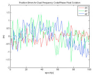
Assuming we have done everything correctly, we will have what is known as a float solution. Because least squares doesn’t know any better, it estimates the integer ambiguities to be real-valued numbers, which we know to be untrue. The accuracy of the float solution is shown below for 100 epochs of data.
float

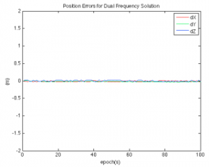
Looking at the figure above, we can see the accuracy of the float solution is generally on the order of 0.5-2m, a significant improvement from absolute positioning. However, its not 2-5 cm accuracy we expect from survey grade GPS receivers! So how do we improve the float solution so that we can achieve higher accuracies(such as the plot below)?
Screen Shot 2013-01-28 at 1.13.03 AM

Stay tuned!

In land surveying, navigation, and photogrammetry, we often take high quality GPS position solutions for granted. Real-time position solutions at centimeter level have become routine, in fact, we may even feel entitled to it. However, as many of you know, and I’ve recently found out, designing a software architecture and embedding the entire GPS solution process within is no trivial task.  In particular, we must ask the question, how exactly does one obtain cm level positions from a satellite broadcasting a signal 20,000 km above the earth? The following series of posts will hopefully elucidate different GPS algorithms and observations and their associated accuracies. I’ll be using LaTeX for the first time, so bear with me…

In order to obtain cm level positioning capabilities, we must employ differencing techniques, that is, we must use multiple receivers and difference the observations obtained with the receiver at a known position with the observations obtained with a receiver at the unknown location (the rover) in order to improve the accuracy of the position solution. It simply isn’t possible to obtain real-time positions on the cm level using a single autonomous receiver and observations available to civilians. Additionally, it is fairly difficult to achieve cm level positioning using single frequency receivers as well, as we will soon see. However, with dual frequency receivers, this is possible, though of course more expensive as well.

“Why do we need to difference GPS measurements made at multiple sites” you may ask? Well, there are many errors (e.g. satellite position, receiver clock offset, etc) that are included in the GPS observations. If the errors at both receivers are constant values, they can be removed using differencing operations. There are several differencing operations, such as single, double, and triple, however, the next few blog posts will focus entirely on double differencing using code and carrier phase observations.

Stay tuned!

Hi Everyone (who may eventually read this),

This blog is meant to serve as an outlet for the many different, and oftentimes crazy, ideas which come about in my working, recreational, and perhaps (sigh) personal life.

A quick bio for those who may not know me.  I am a Ph. D candidate within the Geodesy and Geodetic Science dept. at The Ohio State University.  I graduated from  Purdue University with M.S. in Geomatics Engineering, and Ferris State University (MI) with a Bachelor of Science in Surveying Engineering.

As the blog name indicates, I enjoy learning and practicing the science of navigation and positioning.  However, this blog will most likely include a wide variety of of research topics which are on my mind at any given moment.  A quick list of technical topics that will most likely be included in future posts are the following.

1.  Remote Sensing – Passive and active microwave, multi-spectral, etc.

2.  Photogrammetry/ Computer Vision

3.  GPS Positioning

4.  Inertial Navigation with IMU

5.  Unmanned Aerial Vehicle Applications

Hope you enjoy!

Ben Vander Jagt

Create your own website, free on WordPress.com.Create your own website.
Start free